User guide
The Plant NLRscape webserver user guide encompasses aspects regarding the data acquisition and analysis pipelines applied in generating the database and informs the user on how to use the integrated analysis tools and the interactive graphical features.
Summary
- 0. Website structure
- 1. Top-down : Exploring predefined clusters
- 1.1. Clustering by domain organisation
- 1.2. Domain organisation view page
- 1.3. Clustering by homology
- 1.4. Clustering by taxonomic spread
- 1.5. Cluster view page
- 2. Bottom-up: Start from your sequence of interest
- 3. General domain statistics
- 4. Data download and file formats
- 5. References
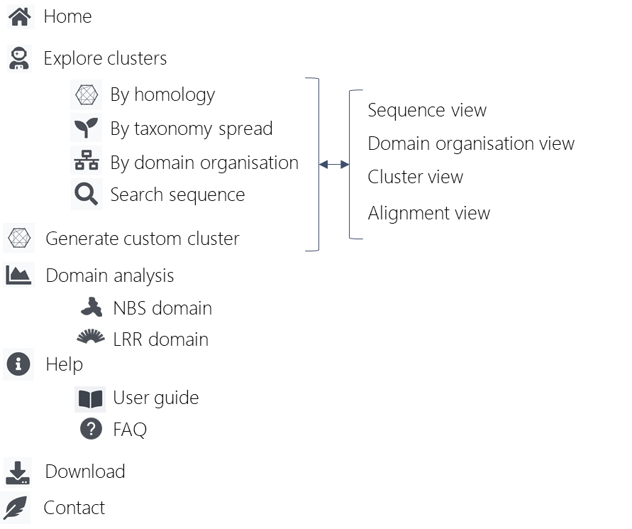
0. Website structure
The Diagram below shows the overall organization of the website :
1. Top-down: Exploring predefined clusters
1.1. Clustering by domain organisation
Plant NLRscape atlas currently contains a collection of aprox. 80.000 plant proteins from UniprotKB that contain NBS-like domains. These sequences were subjected to domain delination using both in-house mapping (HMM-based using HMMER suite (Potter et al., 2018), as well as the available existing annotations in the Interpro collection (Mitchell et al., 2019).
Based on the domain organisation, sequences where classified into the following NLR classes:
- Established NLR classes:
- CNL : with the canonical CC-NBS-LRR organisation
- TNL : with the canonical TIR-NBS-LRR organisation
- RNL : with the canonical RPW8-NBS-LRR organisation
- Residual classes:
- NL : NBS & LRR domains, but no CC / TIR / RPW8
- NBS : NBS domain and no other NLR associated domains.
- Canonical core : with the canonical class organisation ( CC/TIR/RPW8 - NBS - LRR )
- Canonical core + marginal domains : At the N-ter / C-ter margins of the canonical core, additional domains are present
- Incomplete core: missing NBS subdomains or LRR domain.
- Atypical : containing multiple or incomplete NBS domains
Within the first half of the domain organisation page, a summarising diagram of the Plant NLRscape domain stats can be inspected. The second half of the page consists of a table where users can select specific domains and search for a particular domain or organisation or other keywords.
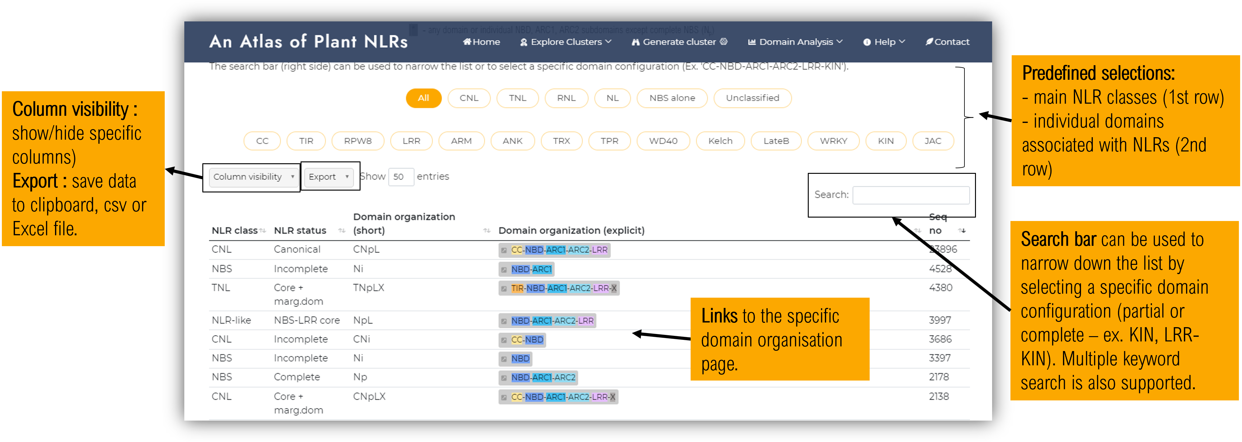
Clicking on a specific domain organisation link, a detailed domain organisation viusalisation page will open, as described bellow.
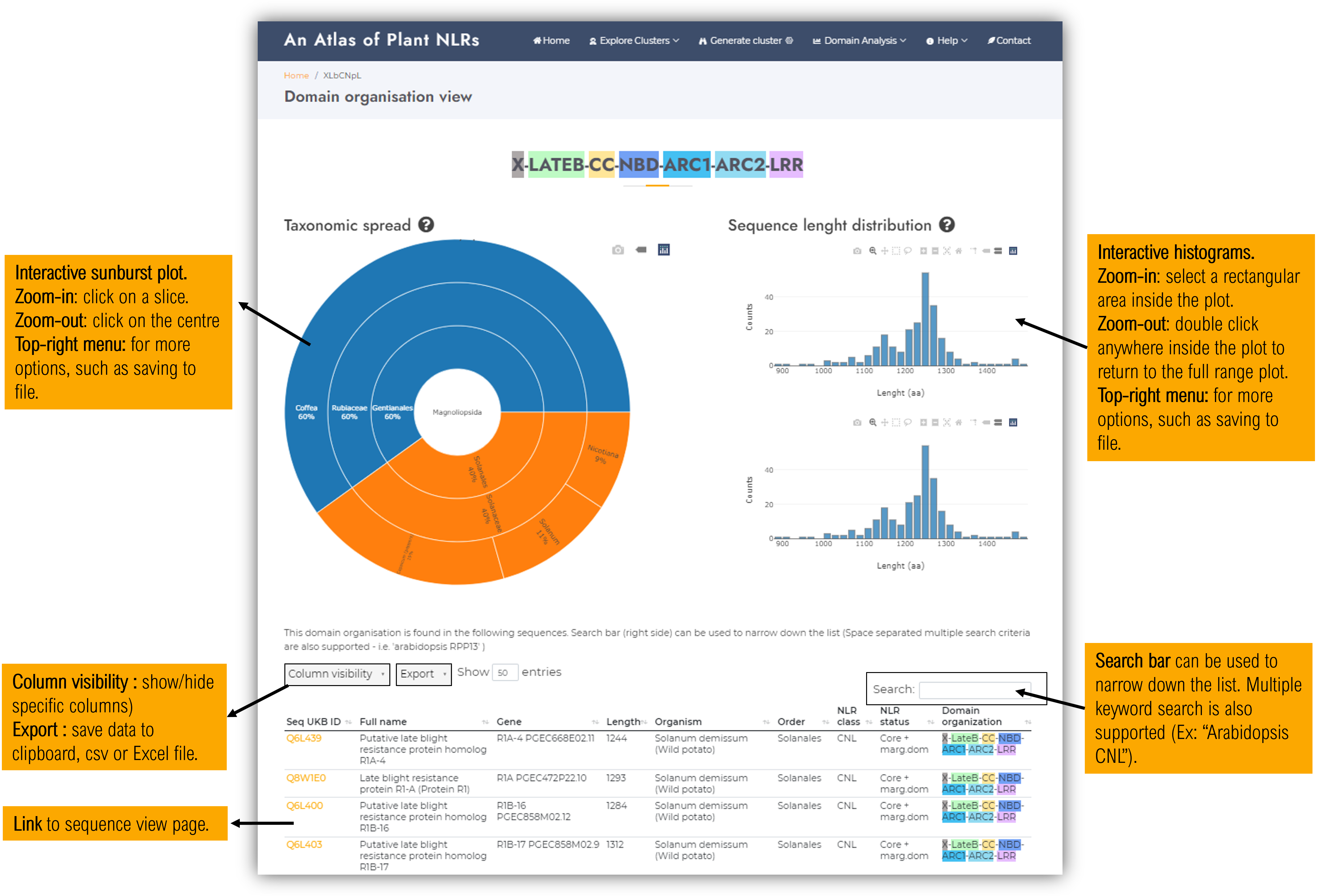
1.2. Domain organisation view page
The domain organisation visualisation page contains info regarding the sequences containing this domain architecture:
- Taxonomic spread sunburst plot
- Sequence lenght distribution : all and nonredundant (90% identity) sequences.
- Sequence data table.
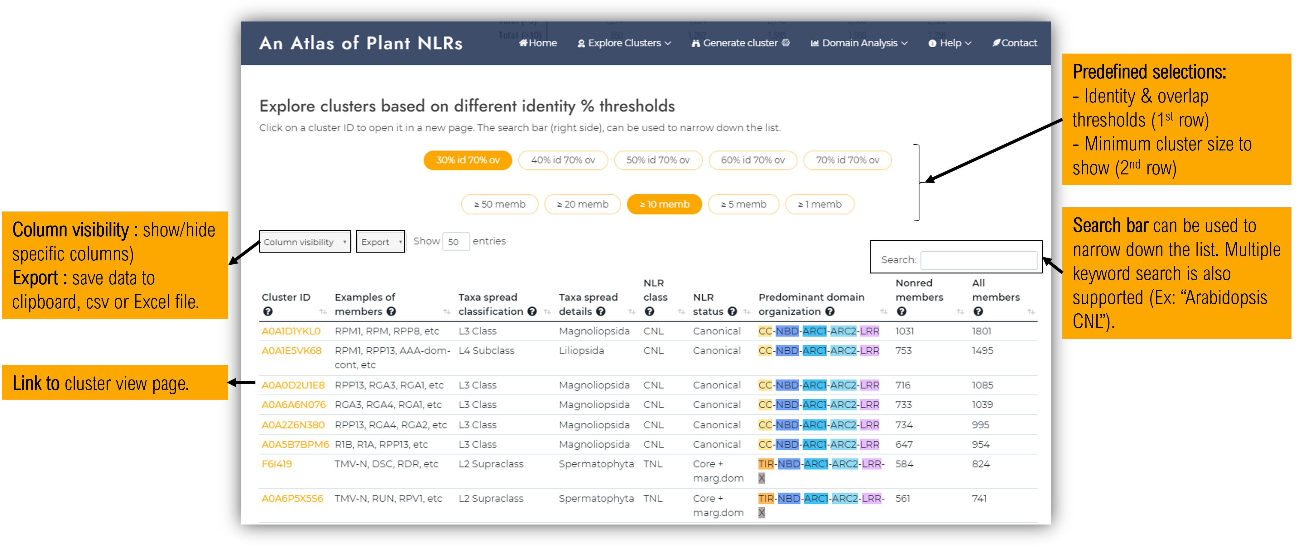
1.3. Clustering by homology
The potential NLR sequences gathered within Plant NLRscape were clustered at different identity (30-90%) and overlap (70/90%) thresholds using MMseqs2 (Steinegger & Söding, 2017). A comprehensive report of the methodology used for clustering is covered within the publication (link will be available soon).
Briefly, the homology cluster signifies a group of sequences sharing similarity above the identity and coverage percentages used as cutoff. For each cluster a sequence representative is selected as the cluster center being the sequence with the most connections (number of sequences having an identity percent higher than the cutoff). The UniprotKB ID of this sequence representative will further on be designated as the cluster ID.
The homology clusters page contains three sections, as follows :- Interactive graph representation of clusters (only for 30% identity & 70% overlap cutoffs due to the large number of clusters for less restrictive cutoffs)
- Clusters size histograms.
- Clusters data table.
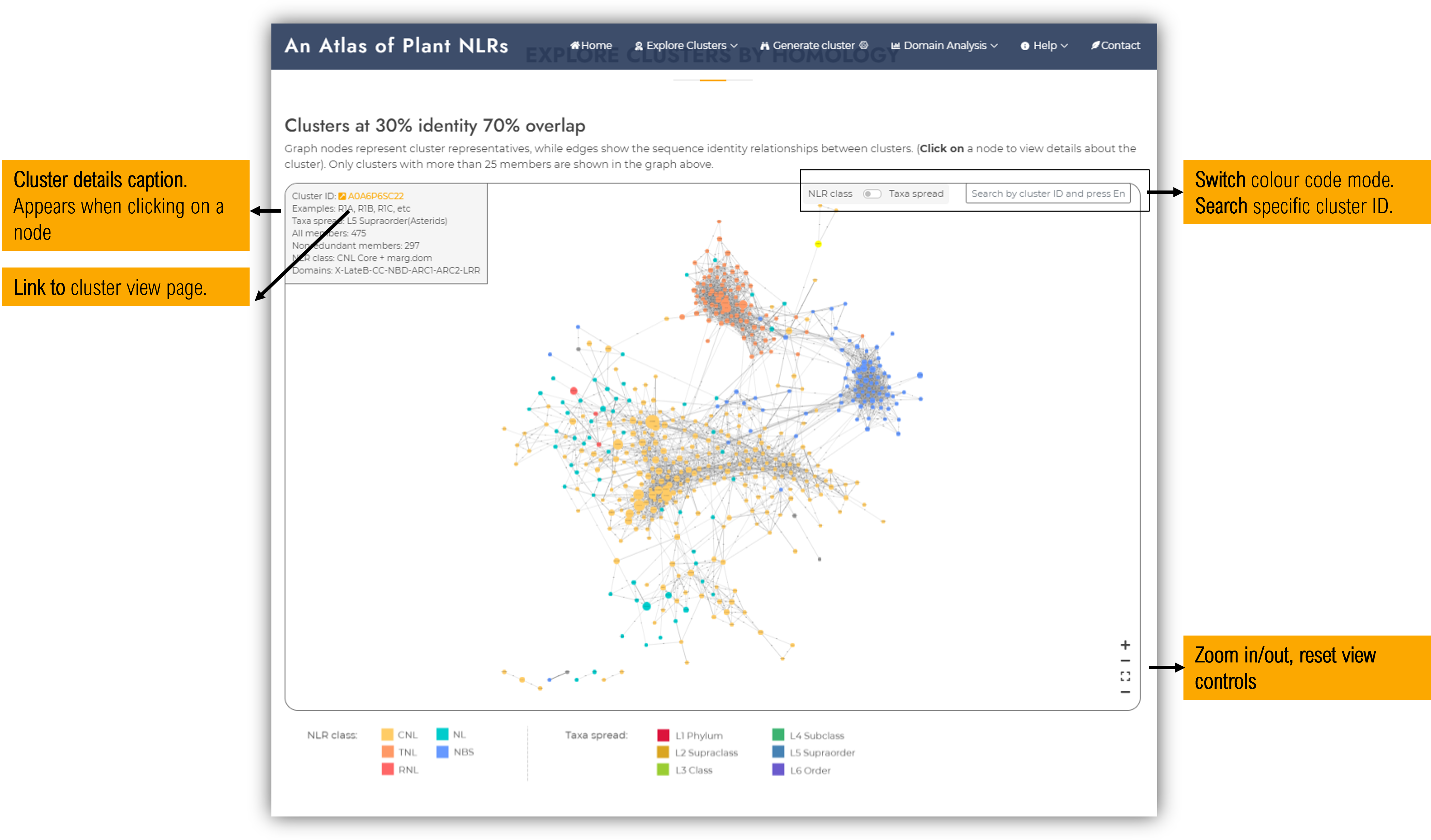
Cluster graph
Graph nodes represent cluster representatives, while edges show the sequence identity relationships between clusters. By clicking on a specific node, a caption with cluster details will appear in the top-left side of the graph window. Only clusters with more than 25 members are included in this graph, in order to ease visualisation. Separately, on each cluster visualisation page, a subgraph of its neighbour clusters can be further examined.
Limitations: The graph representation tries to find the best 2D projection using as edge lenght the identity percent between two cluster representatives by employing an edge-weigthed spring embedded layout solver implemented in Cytoscape (Franz et al., 2016; Shannon et al., 2003). As the protein space is highly dimensional, a 2D representation of all these relationships cannot be perfectly achieved, therefore we recommand inspecting the identity values shown on each edge label to avoid misleading interpretations. Such a 2D representation is recomanded only for a general perspective of relationships between NLR main groups.
Clusters data table
Clusters at different identity % thresholds can be examined within the data table. The search bar (top-right side) can be used to narrow down the list and it also supports multiple keyword searches.
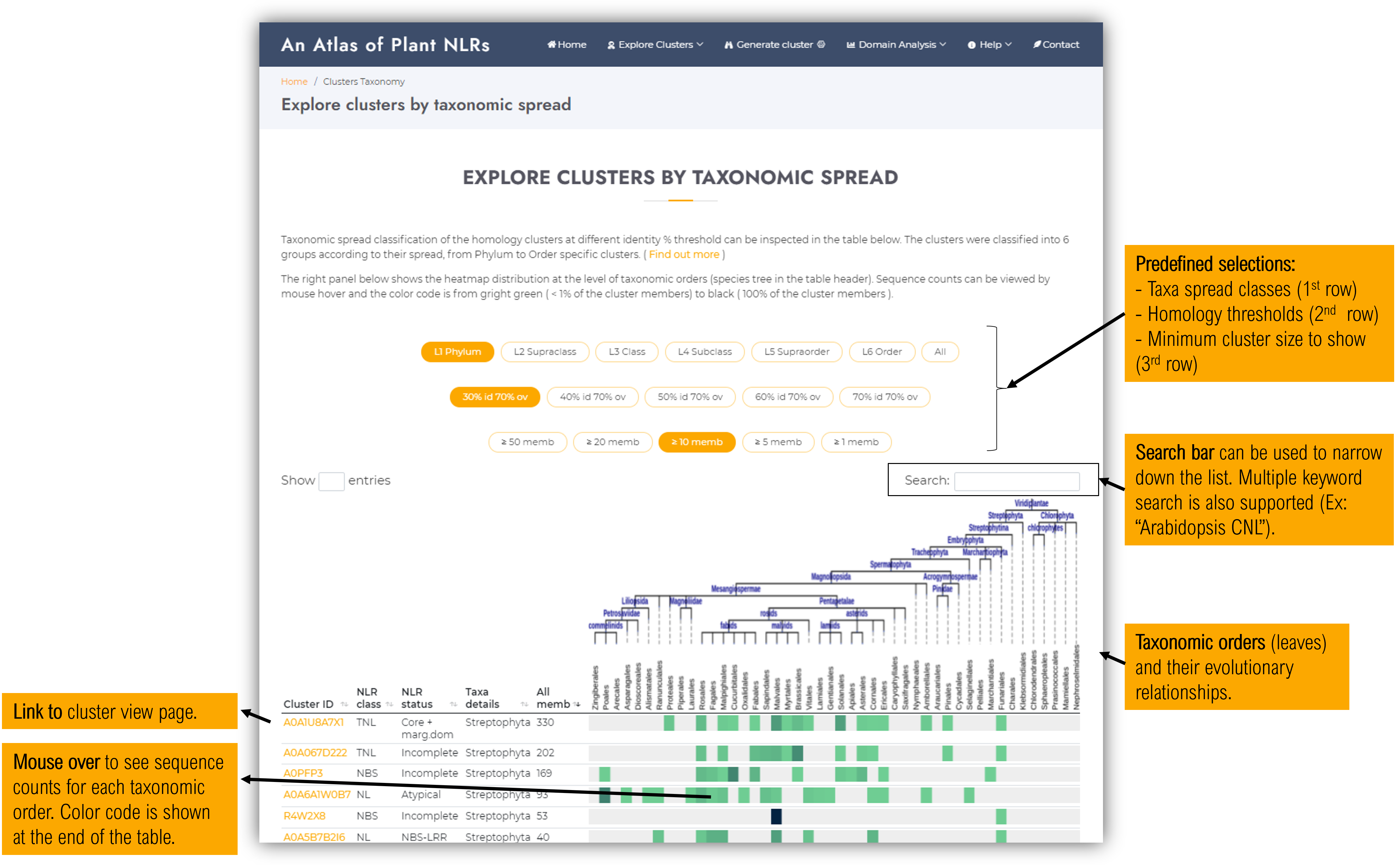
1.4. Clustering by taxonomic spread
The homology clusters were classified into 7 groups according to their spread, from Kingdom- to Order- specific clusters. However, kingdom-spread clusters were not found within the current NLR collection, the most taxonomically spread cluster being of type Phylum. The diagram below shows the taxonomic groups taken into account at each spread level.
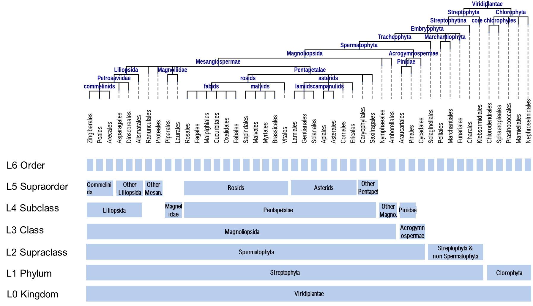
Please note that the evolutionary tree above shows only the orders where NLR-like sequence were found and not all the taxonomic orders within the Viridiplantae kingdom.
Within this page, users can examine the taxonomic spread classification of the homology clusters at different identity % threshold.
The right panel shows the heatmap distribution at the level of taxonomic orders (species tree shown in the table header). Sequence counts can be viewed by mouse hover and the color code is from light green (<1% of the cluster members) to black (100% of the cluster members), as indicated by the color scale diagram below the table.
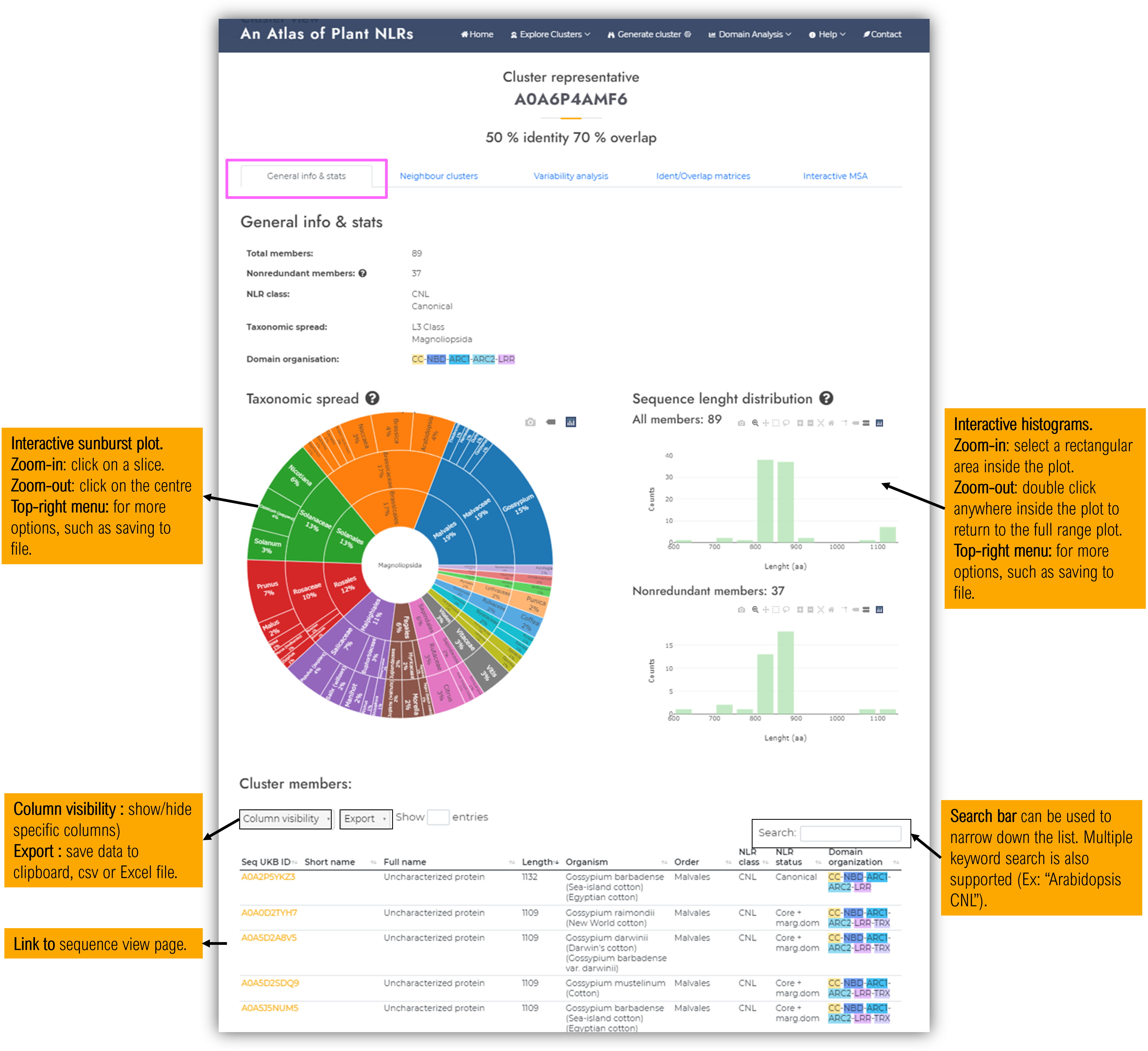
1.5. Cluster view page
The cluster visualisation page comprises a series of data and bioinformatic analyses outline which can be visualised with in-browser interactive tools. These data can be accessed for each predefined homology cluster generated using different sequence identity thresholds (30%-70%) by clicking on the cluster ID link within other pages of the Atlas. The cluster visualisation page is structured in the following subsections (tabs):
- General info and stats.
- Neighbour clusters graph.
- Variability analysis.
- Identity / Overlap matrices.
- Interactive MSA.
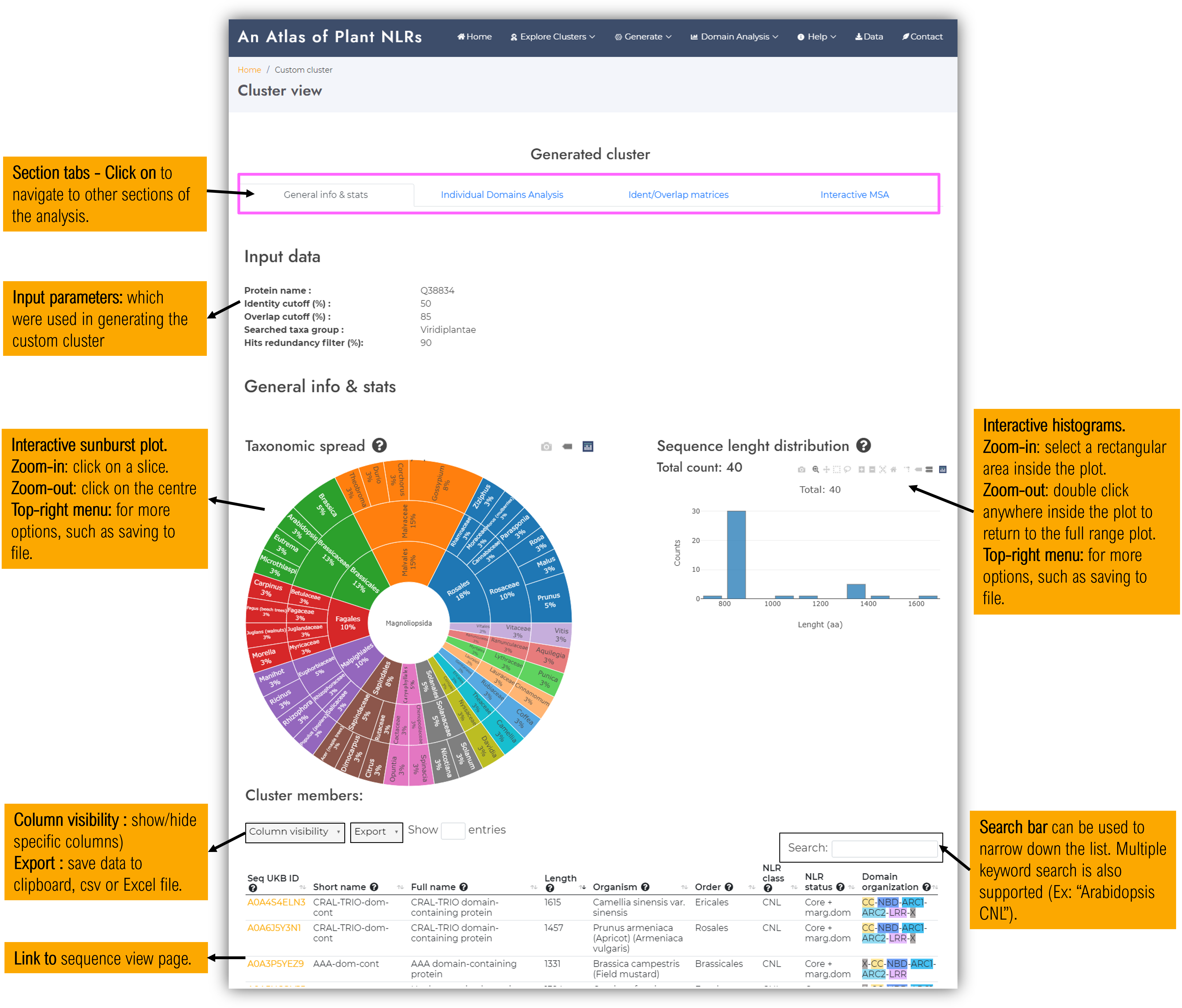
1.5.1 General info & stats tab
As stated from its name, the first tab shows general cluster data :- Generic stats :
- Member count (all / only nonredundant)
- Predominant NLR class (the most often occuring NLR class among its members)
- Taxa spread class
- Predominant domain organisation (the most often occuring domain organisation among its members)
- Taxonomic spread interactive chart
- Interactive sequence lengh distributions (for either all cluster members, or a selection containing only nonredundant members < 90% identity)
- Interactive cluster member table - which containes details about each cluster sequence member (including links to sequence visualisation pages).
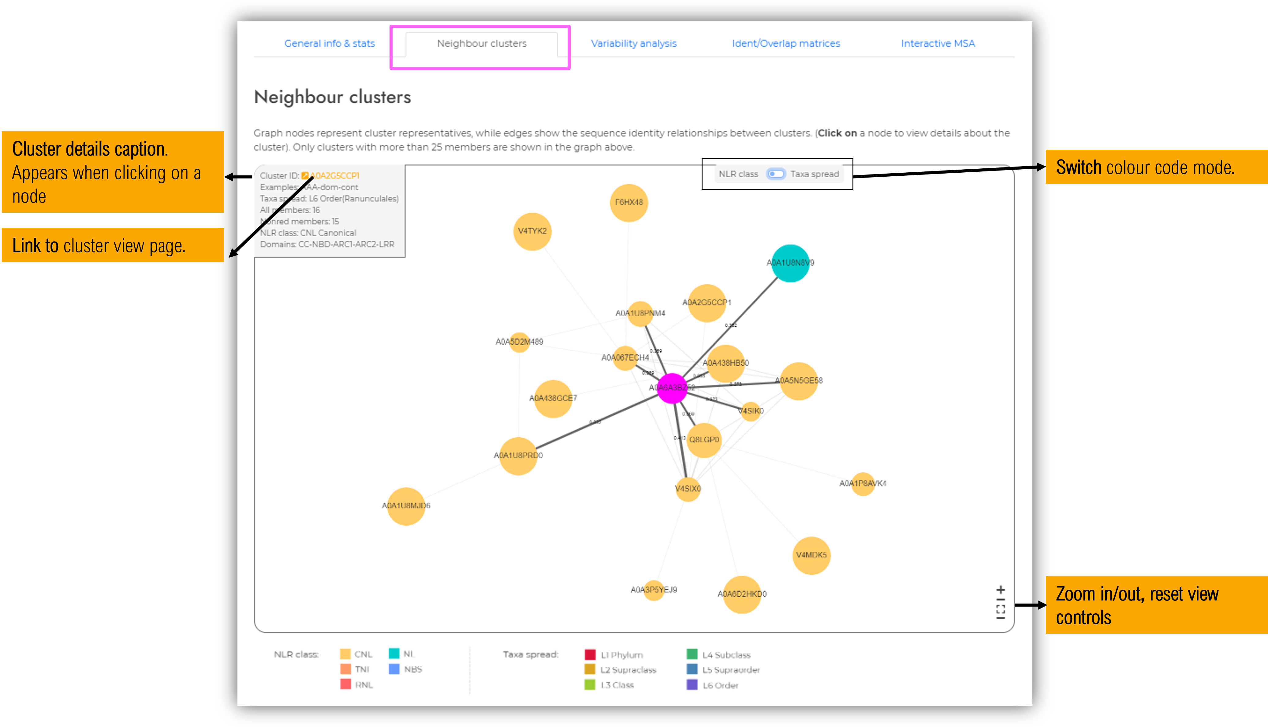
1.5.2 Neighbour clusters tab
Graph nodes represent cluster representatives, while edges show the sequence identity relationships between clusters. By clicking on a specific node, a caption with cluster details will appear in the top-left side of the graph window. In order to ease visualisation, for each identity homology cutoff value, we selected custom parameters for subgraph representation in order to get a good balance between the relevance of the data and the complexity of the displayed figure. These custom display settings are indicated below the graph panel.
Limitations: The graph representation tries to find the best 2D projection using as edge lenght the identity percent between two cluster representatives by employing an edge-weigthed spring embedded layout solver implemented in Cytoscape (Franz et al., 2016; Shannon et al., 2003). As the protein space is highly dimensional, a 2D representation of all these relationships cannot be perfectly achieved, therefore we recommand inspecting the identity values shown on each edge label to avoid misleading interpretations. Such a 2D representation is recomanded only for a general perspective of relationships between NLR main groups.
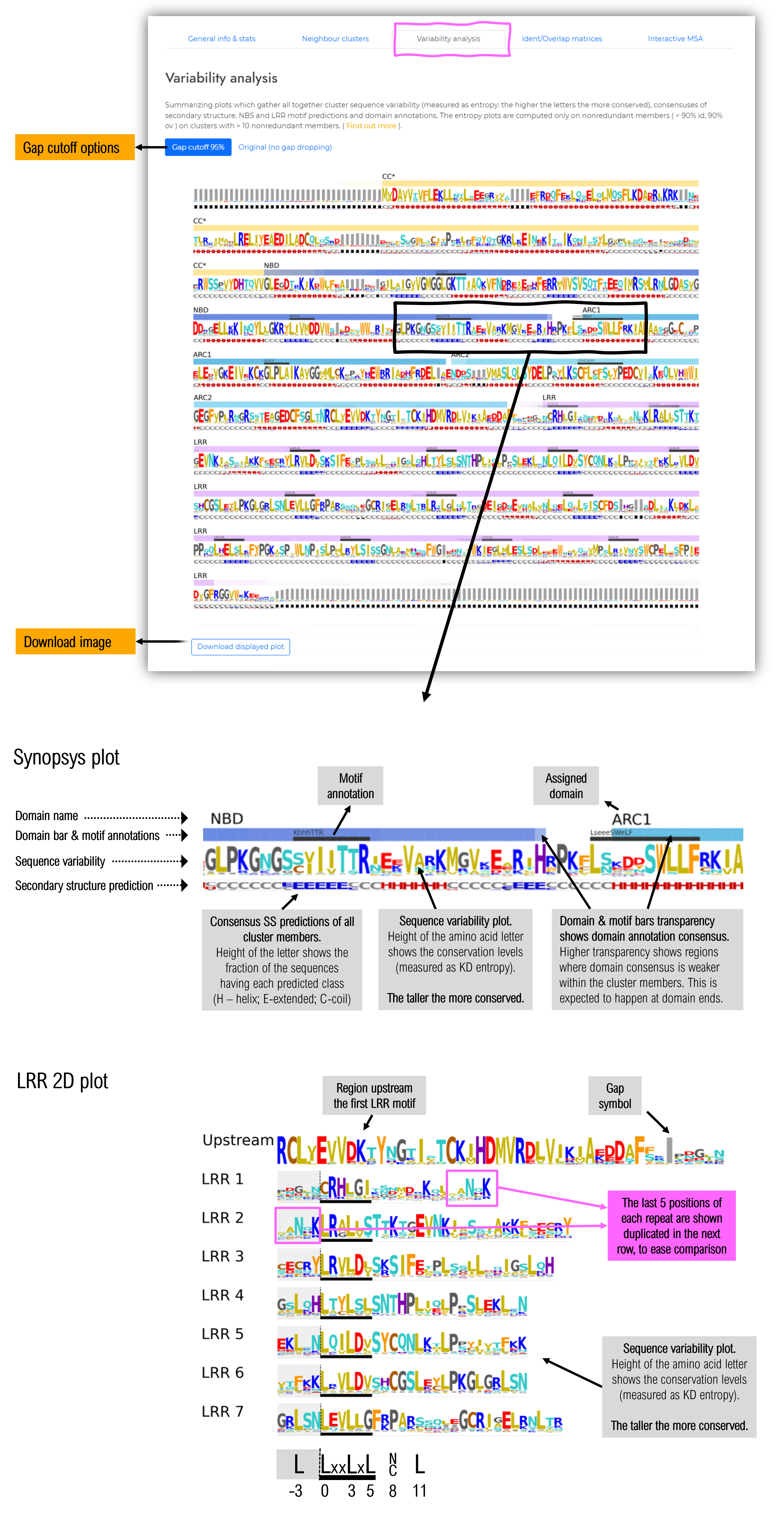
1.5.3 Variability analysis tab
The first half of the page contains a summarising plot of the full sequence, containing data about sequence variability, secondary structure prediction consensus, mapped domains and sequence motifs.
The second half of the page contains a 2D plot showing the LRR repeats arranged one below the other similarly to their 3D arrangement. This layout facilitates the visualisation of the relationships between residues located on consecutive LRR repeats, but in close proximity in the 3D space.
For each type of plot, two options are available:
- Gap cutoff 95%: position of the alignment at which more than 95% of the sequence contain a gap are removed from the plot. This option is usefull for having an overall perspective of the conserved areas and their consensus. This option is particularly helpfull for large clusters at lower homology levels (30-40% identity).
- Original (no gap dropping) : usefull in having a detailed account to where insertions occur within the protein
Within the LRR domain 2D plot are shown only the repeats where there is a strong consensus in LRR motif delination ( the displayed LRR motifs have a LRR motif prediction in more than 40% of sequences comprising the cluster).
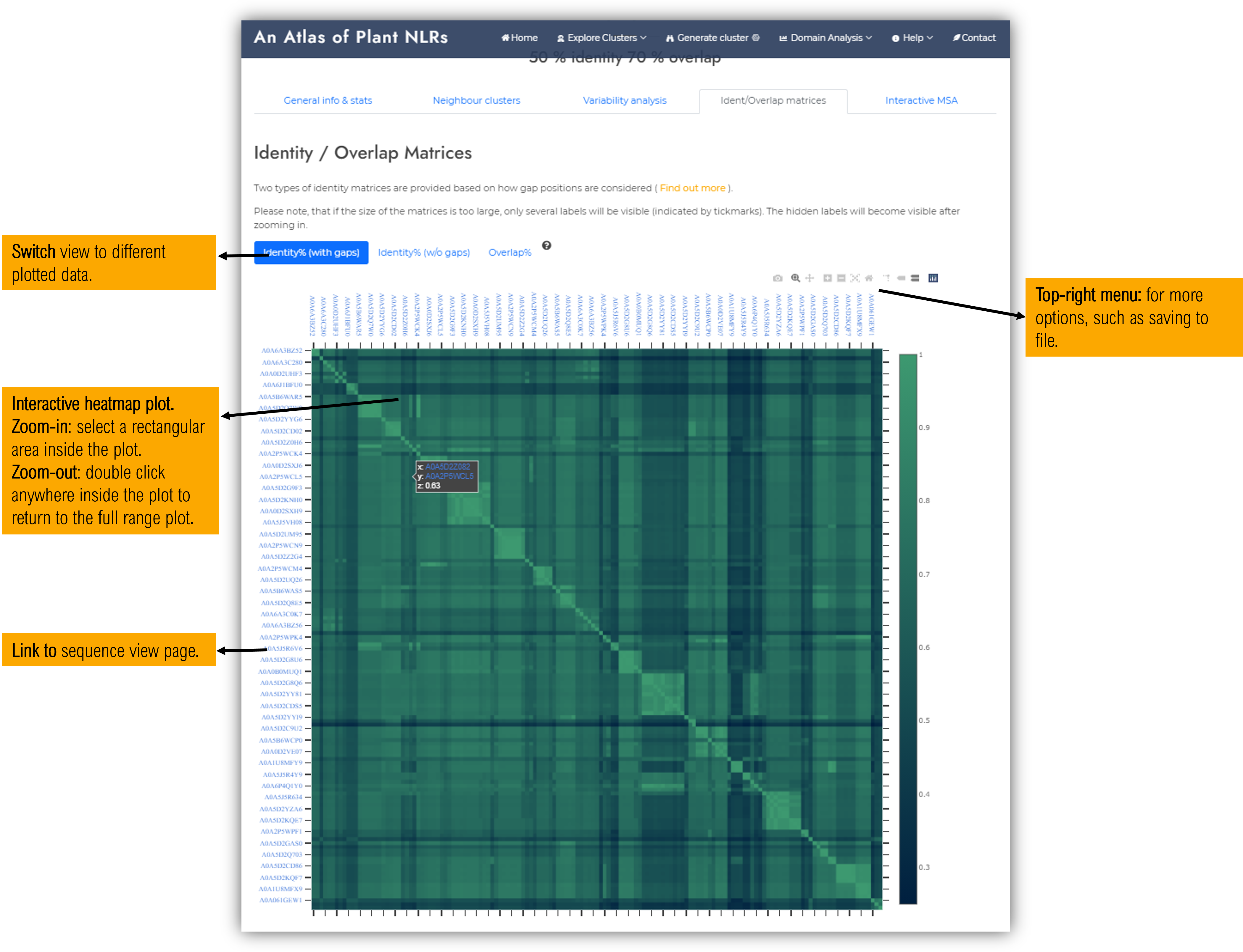
1.5.4 Identity / Overlap matrices tab
This tab contains identity / overlap matrices of the cluster members, showing the intra-cluster relationships and how sequences further group based on sequence homology.
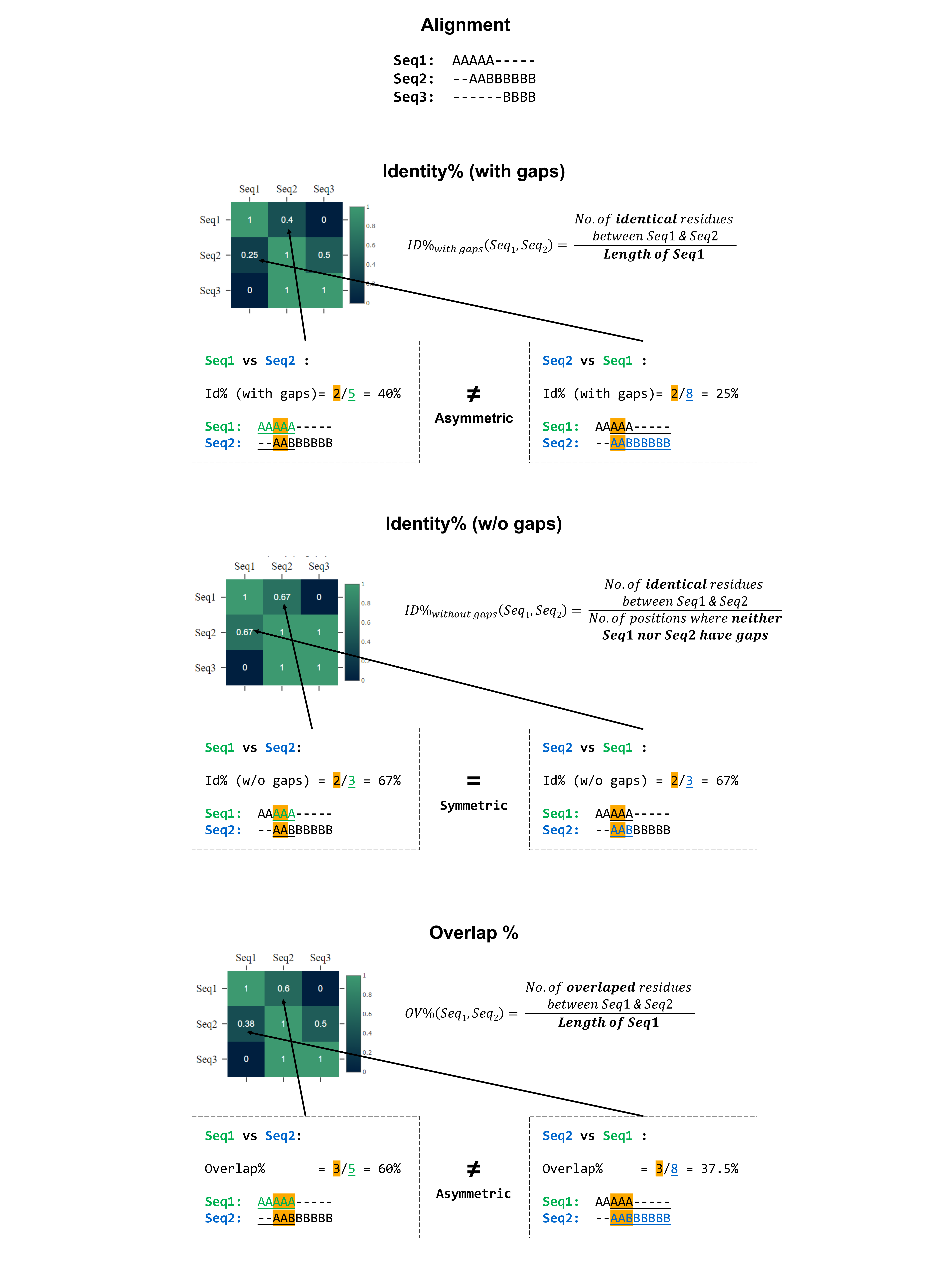
Three types of matrices can be visualized:
- Identity % with gaps - taking gap position into account
- Identity % without gaps - does not take gap position into account, but only positions where both sequences have aligned amino acids.
- Overlap % - shows the percentages of the sequence aligned with the other one.
Two types of identity matrices are provided based on wether the gap positions are considered. The equations and an illustrative example is provided below:
Please note that if the cluster contains more than 300 sequence members, the matrices will be open in a separate page upon clicking on the corresponding button. Also, if the size of the matrices is too large, only several labels will be visible (indicated by tickmarks). The hidden labels will become visible after zooming in.
1.5.5 Interactive Multiple sequence alignment (MSA) tab
Cluster members sequence alignments can be inspected online using either of the two provided web apps :
- Our in-house PHP viewer - Suitable for large alignments as it is very fast, but has limited analysis features.
- MSAviewer (Yachdav et al., 2016) - it offers multiple interactive features, but it is not feasible for large clusters.
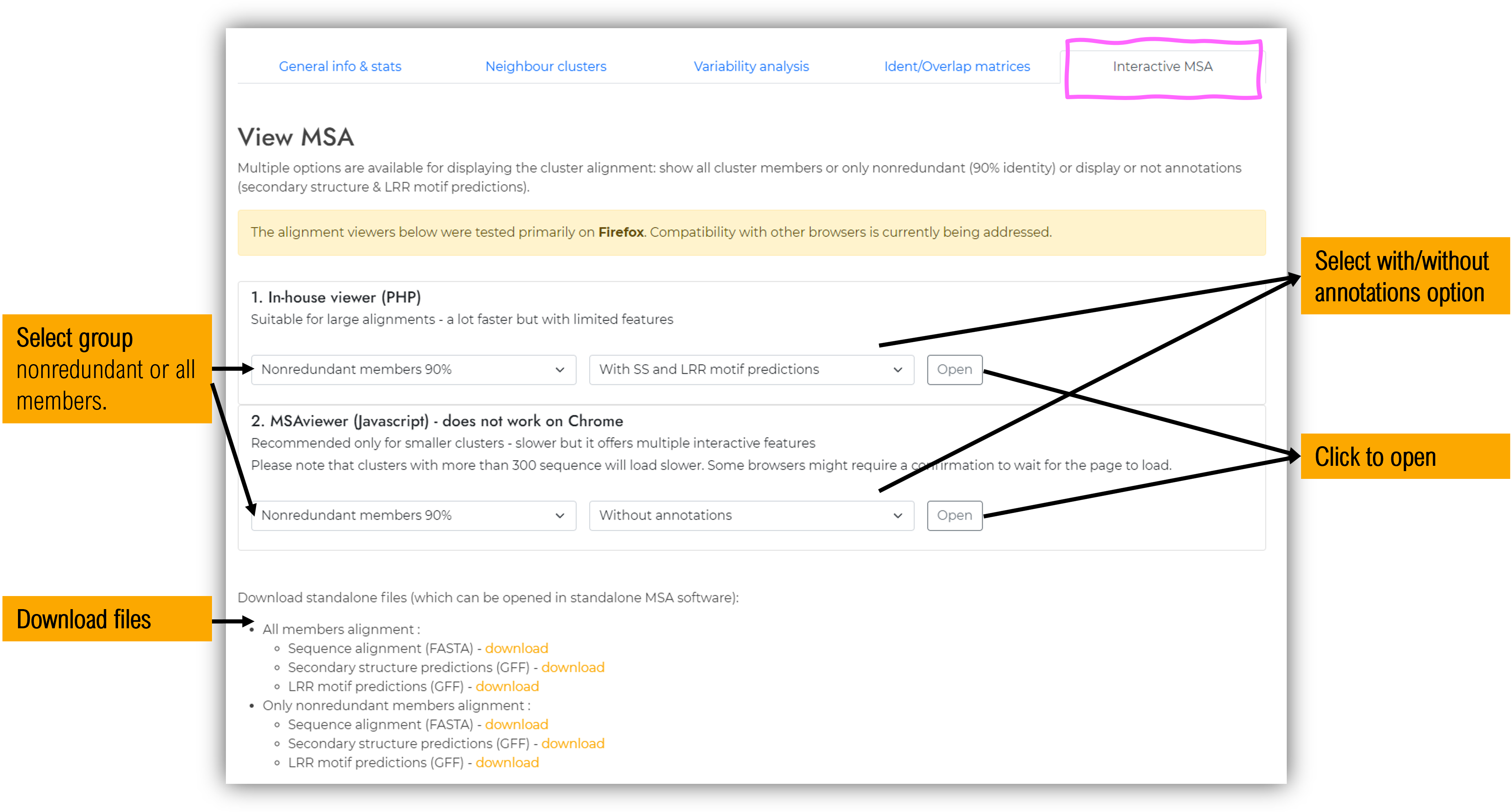
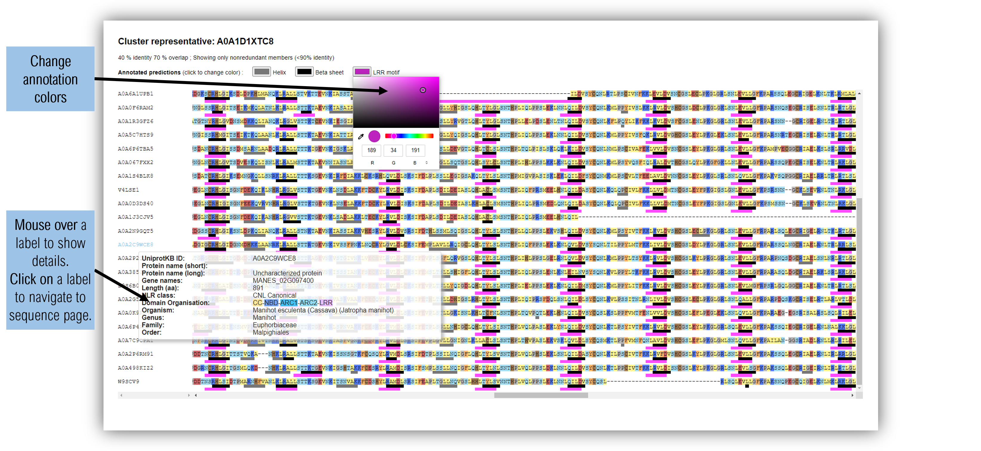
In-house viewer
Faster, but with far less features than MSAViewer. Recommended only for large alignments which do not work well with MSAViewer;
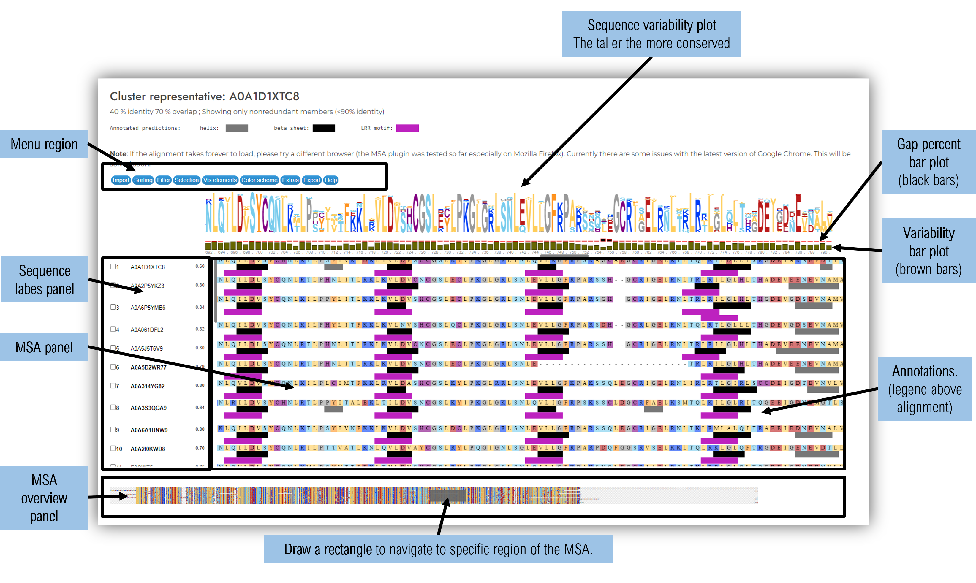
MSAviewer App
MSAViewer (Yachdav et al., 2016) offers multiple interactive features.
Additional info regarding MSAViewer usage can be found within the tutorials and examples they provide : https://msa.biojs.net, https://github.com/wilzbach/msa;
The secondary structure predictions displayed in the plots are computed using RaptorX Predict Property (Wang et al., 2016a, Wang et al., 2016b) and the LRR motif predictions with LRRpredictor (Martin et al., 2020). The alignments are performed using Mafft (Katoh et al., 2013) and the synopsis logos using Logomaker (Tareen et al., 2020).
2. Bottom-up: Start from your sequence of interest
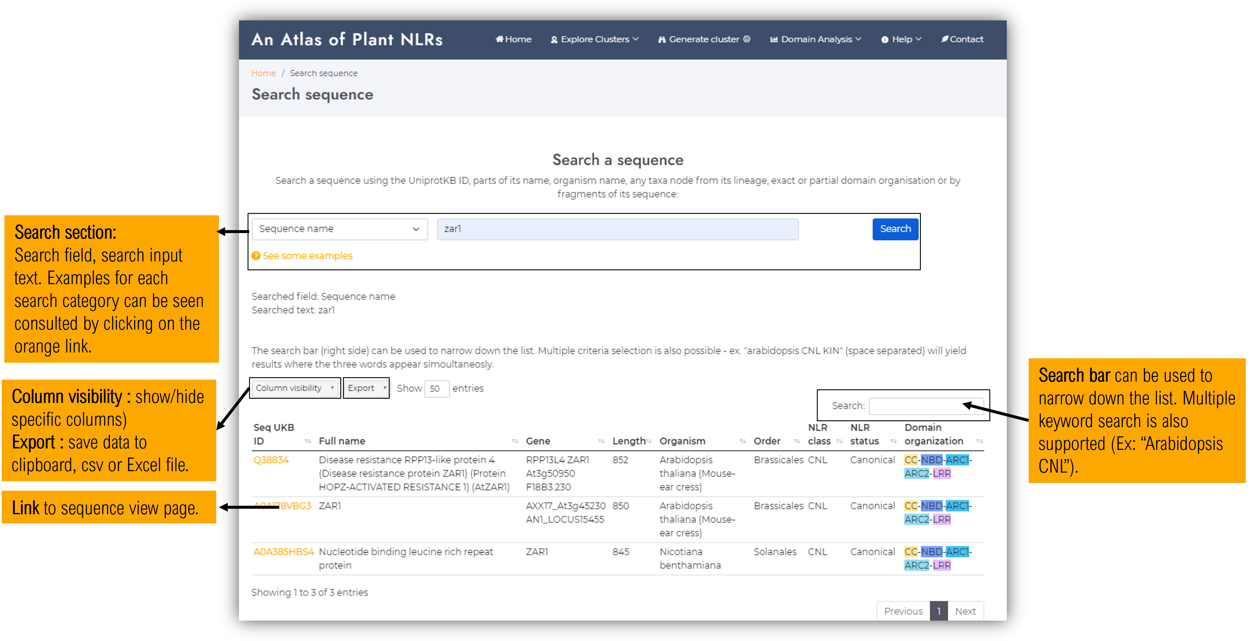
2.1. Search sequence page
Users can query the Plant NLRscape database using specific keywords. The result of the query will be displayed in a table within the lower half of the page. Depending on how wide the search is, querying the database might take between 0-5 seconds. Below are some examples:
-
sequence name"zar1"
-
UKB ID"Q38834" (no spaces)
-
organism name"arabidopsis", "arabidopsis thaliana" (some species have synonym names already integrated, some don't)
-
full lineage"liliopsida", "magnoliopsida", "poales", any internal taxonomic node
-
domain exact organisation"CC-NBD-ARC1-ARC2-LRR", "X-NBD-ARC1-ARC2-LRR-KIN", etc
-
a particular domain or configuration"CC", "RPW8", "KIN", "NBD-ARC1-ARC2", "LRR-WRKY", etc
-
sequence"MVDAVVTVFLEKTLNILEEKGRTVSD" (parts of the sequence with exact match, no spaces / endline characters for the moment)
-
An improved search feature will be available soon, which will also allow blasting sequences for finding close but not identical matches as well.* all search fields are case insensitive.
The results can be further narrowed down using the built-in table search bar (located above the table to the right) which will search only within the table data and will interactively display only the rows matching the inserted keywords. The table search bar also supports multiple keyword search - ex. "potato TNL".
Clicking on a specific sequence ID link, the user will be redirected to the sequence view page.
2.2. Sequence view page
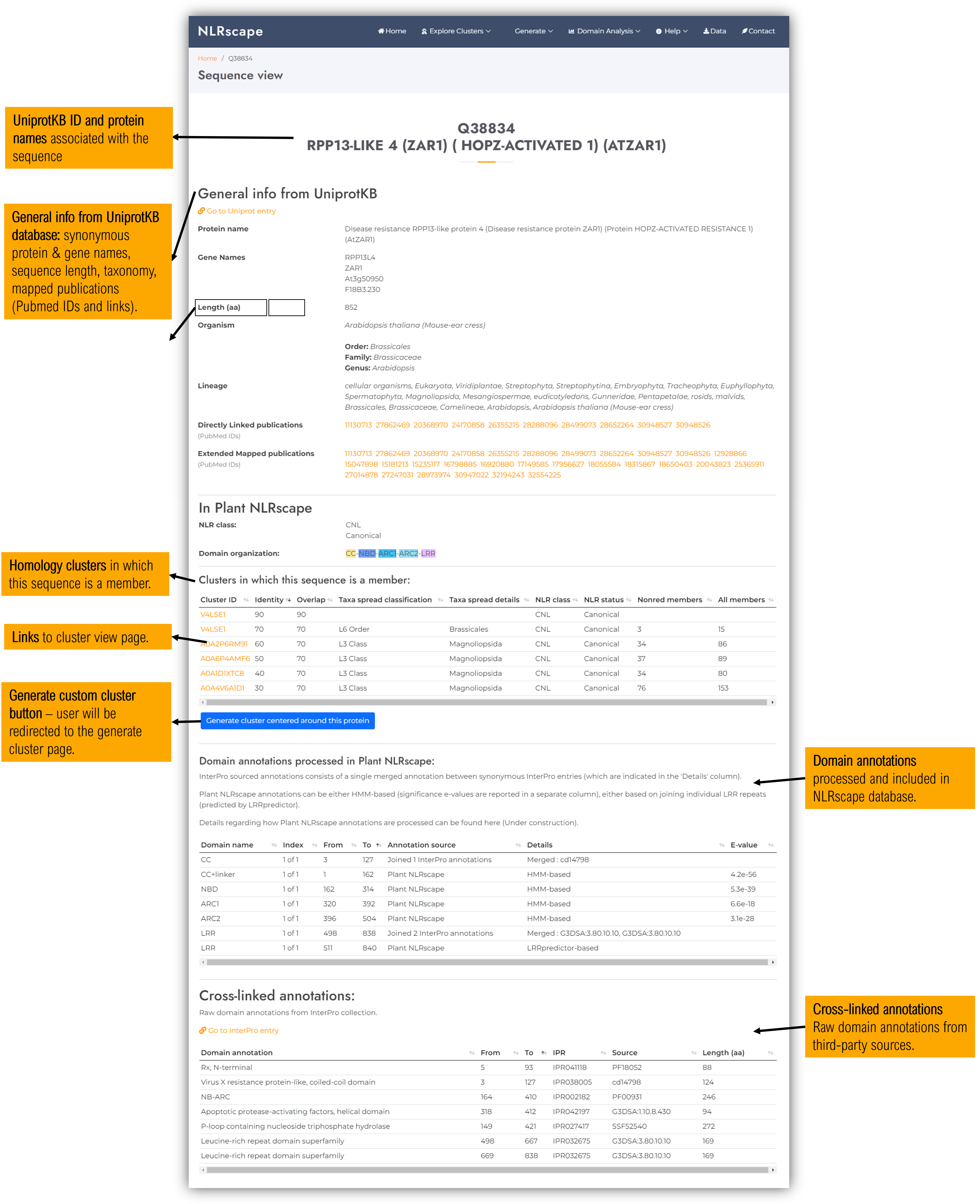
2.3 Generate custom clusters
Besides inspecting the predefined homology clusters at different sequence identity thresholds, users can compute their own clusters centered around a particular protein of interest.
The predefined homology clusters are built by selecting as cluster representative the sequence having the most ‘connections’ (i.e. number of neighbour sequences with identity percents above the threshold). Therefore, if the protein of interest is located at the extremity of the cluster, some of their homologs might be placed in a different cluster. This occurs because the identity relationships landscape is complex, and even though the clustering algorithm (MMseqs2 - Steinegger et al., 2018) tries to find the best space partition of the NLR space, particular clusters might be very ‘close’ to each other.
To overcome this matter, users can generate custom clusters which will build a cluster centered around your protein of interest and will include all homologs above the selected identity and coverage cutoffs.
Moreover, the users can impose constraints on a specific taxonomic branch or particular redundancy levels between the cluster members (i.e. identity percent cutoff to which any member pair should not exceed).
2.3.1 Input form page
This feature can be accessed either from the top menu, but also from the sequence detailed view page. If the later, the entry name and amino acid sequence will be automatically filled. Users can also insert any sequence regardless of wether it is present in the database or not.
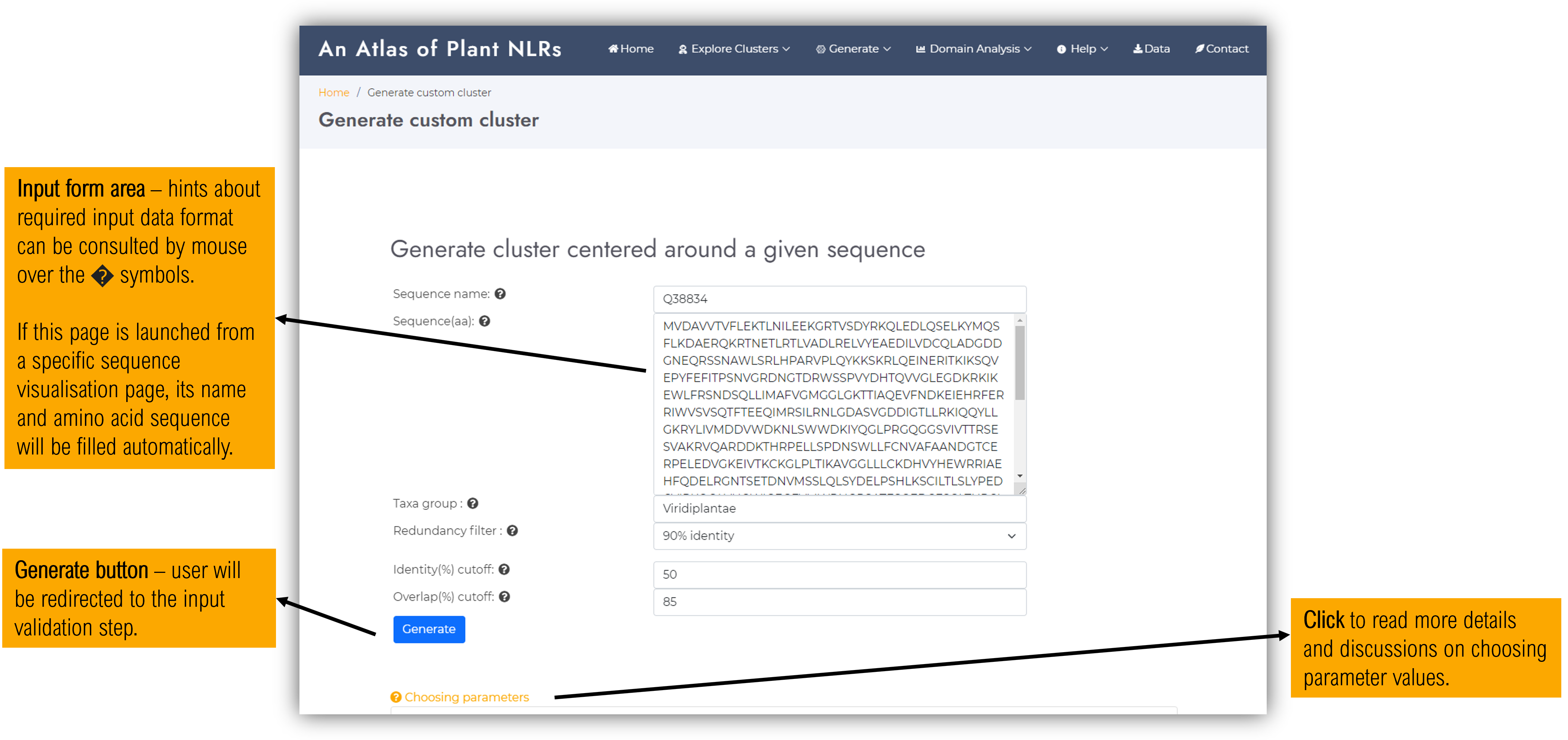
Besides the name and amino acid sequence, user have the following parameters to customize their cluster :
-
Redundancy filterSelect from the database only representatives at a given redundancy level, expressed as identity percent. For example, choosing a redundancy filter of 70% will retrieve only the hits that have less than 70% identity between themselves.
-
Identity(%) cutoffValues can be between 20 and 100. The searched sequences will be gathered to have higher identity percents than the selected cutoff, with respect to the input protein. Choosing a low identity cutoff will yield in a larger and more diverse cluster.
-
Overlap(%) cutoffBetween 20 and 100. The cluster sequences will be gathered to have higher coverage percents than the selected cutoff, with respect to the input protein sequence. Choosing a low value will yield both in retrieving complete and incomplete sequences hits, but also in a more diverse cluster (as the identity % cutoff constraint will apply on any sequence segment percent above the overlap cutoff)".
-
Input sequenceAs input sequence, users can provide either a complete sequence or a fragment corresponding to a particular domain. Depending on the choice, the identity and overlap parameters might require adjustments depending on the case. This can be done after the search step depending on how many sequences are gathered to satisfy the input criteria.
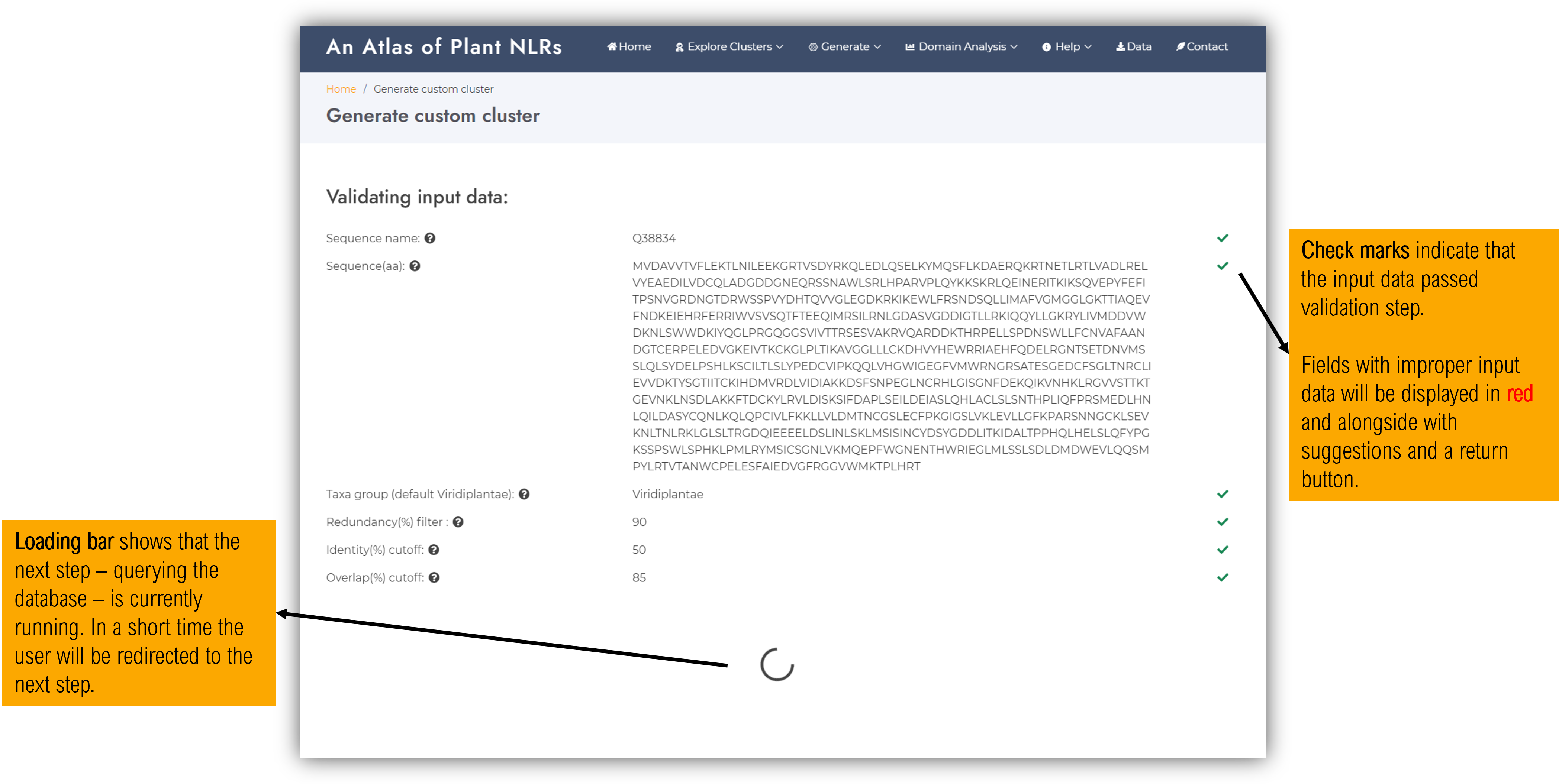
2.3.2. Input validation page
At this step the input data will be checked for compliance. If valid, green check mark symbols will be shown alongside each field and the next step will be launched. Otherwise, the problematic fields will be indicated wih red cross mark symbols and additional info and suggestions will the displayed.
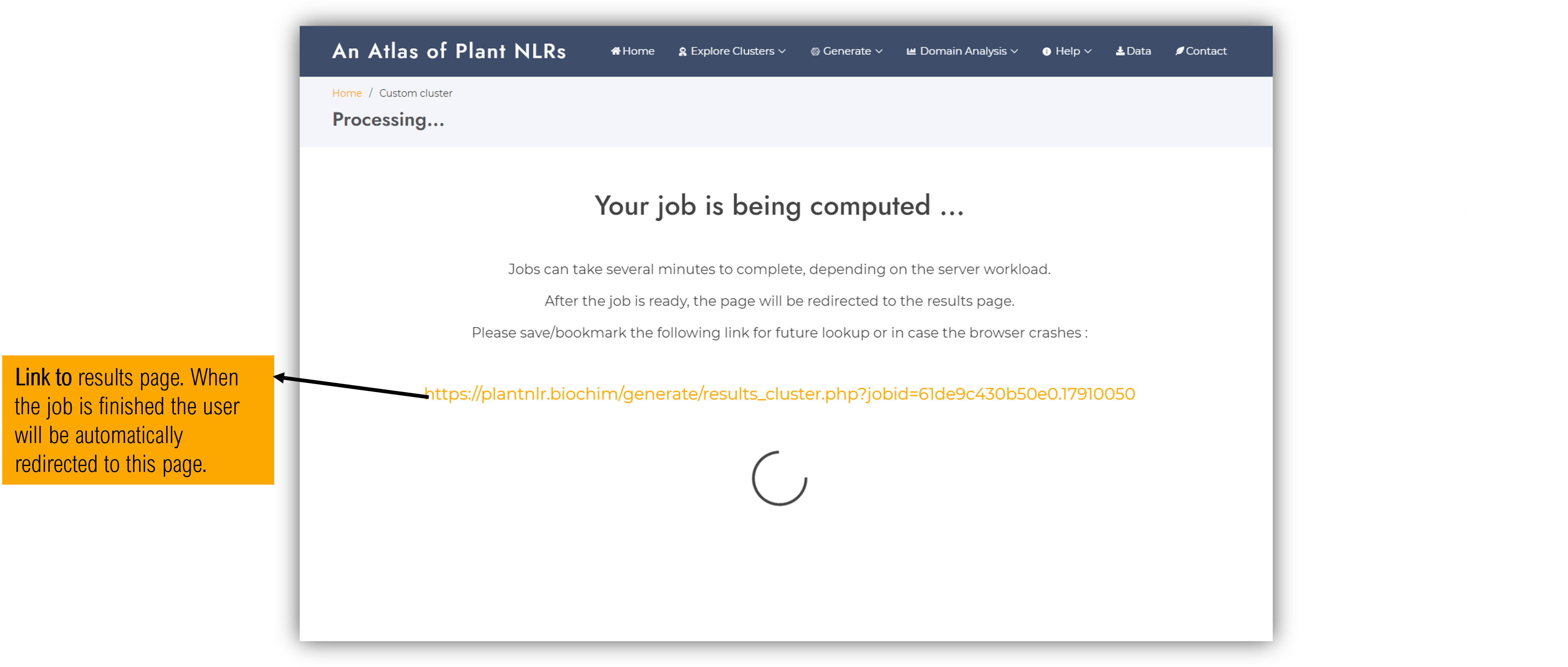
The next stage of the workflow will be automatically launched and while the job processing is udergoing a loading circle will be displayed.
2.3.3. Results part 1: Hits result
At this stage, the plant NLR database has been queried for sequences compliant with the input parameters.
If the resulted hits are too few ( < 20 ) or too many ( > 500 ), we suggest to return and select less / more stringent cutoffs as too small clusters are not statistically significant for variability analysis, while too large clusters might aggregate and dilute distinctive heterogenous sequence properties.
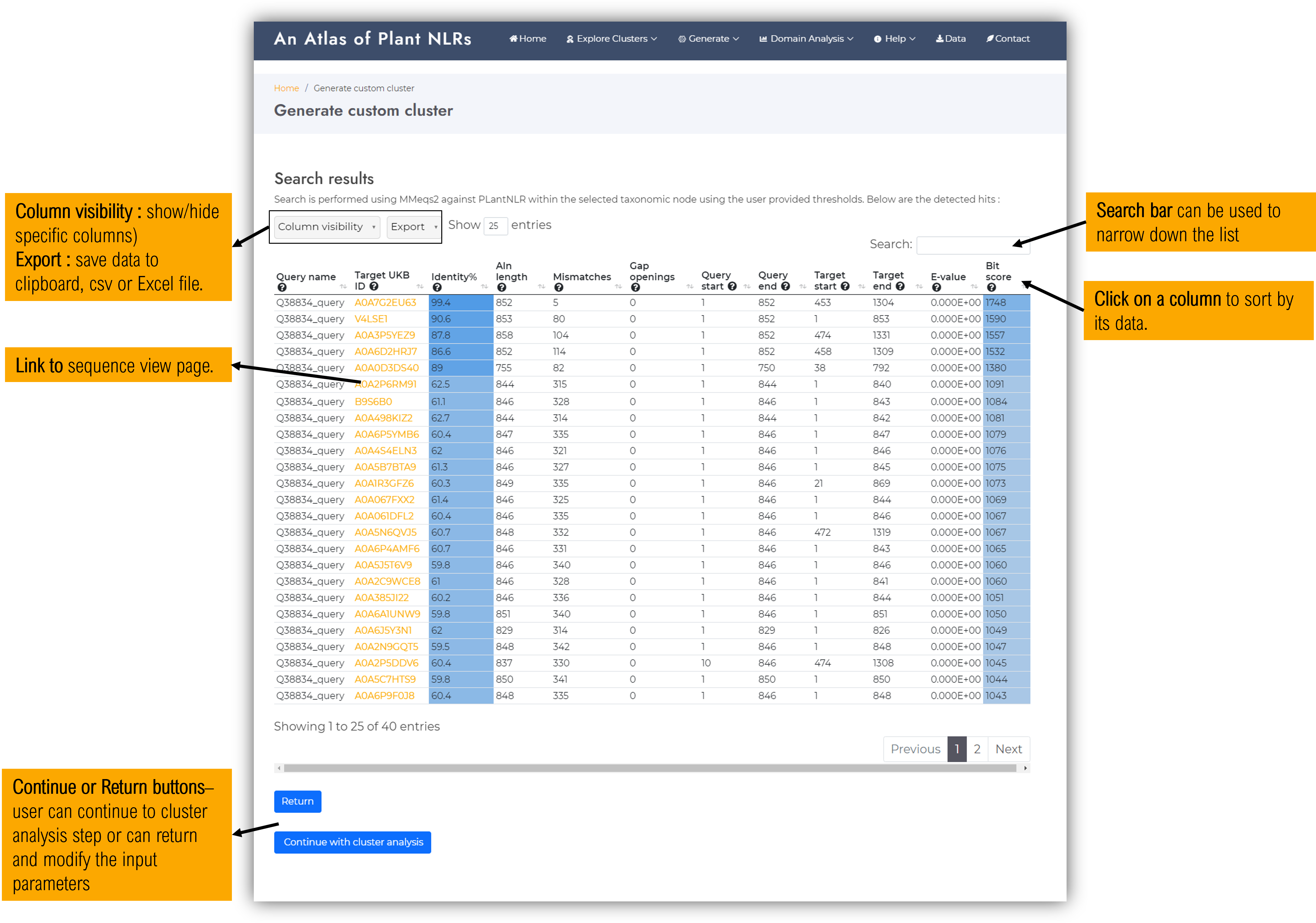
Next step will consist of performing analysis on the identified members.
This stage of the workflow is computational consuming and might take several minutes depending on the size of the cluster and the server workload. The page will automatically be redirected to the final results page when the job is ready.
We suggest users to copy the randomly generate job ID link displayed on the loading screen to further access their results at a later time, or in case the connection is reset by the browser.
2.3.5. Results part 2: Cluster analysis
The analysis of the custom generated cluster is now done !
The visualisation page is almost identical with the predefined clusters view page in terms of organisation and types of displayed data. Please see the corresponding section of the user guide - here.
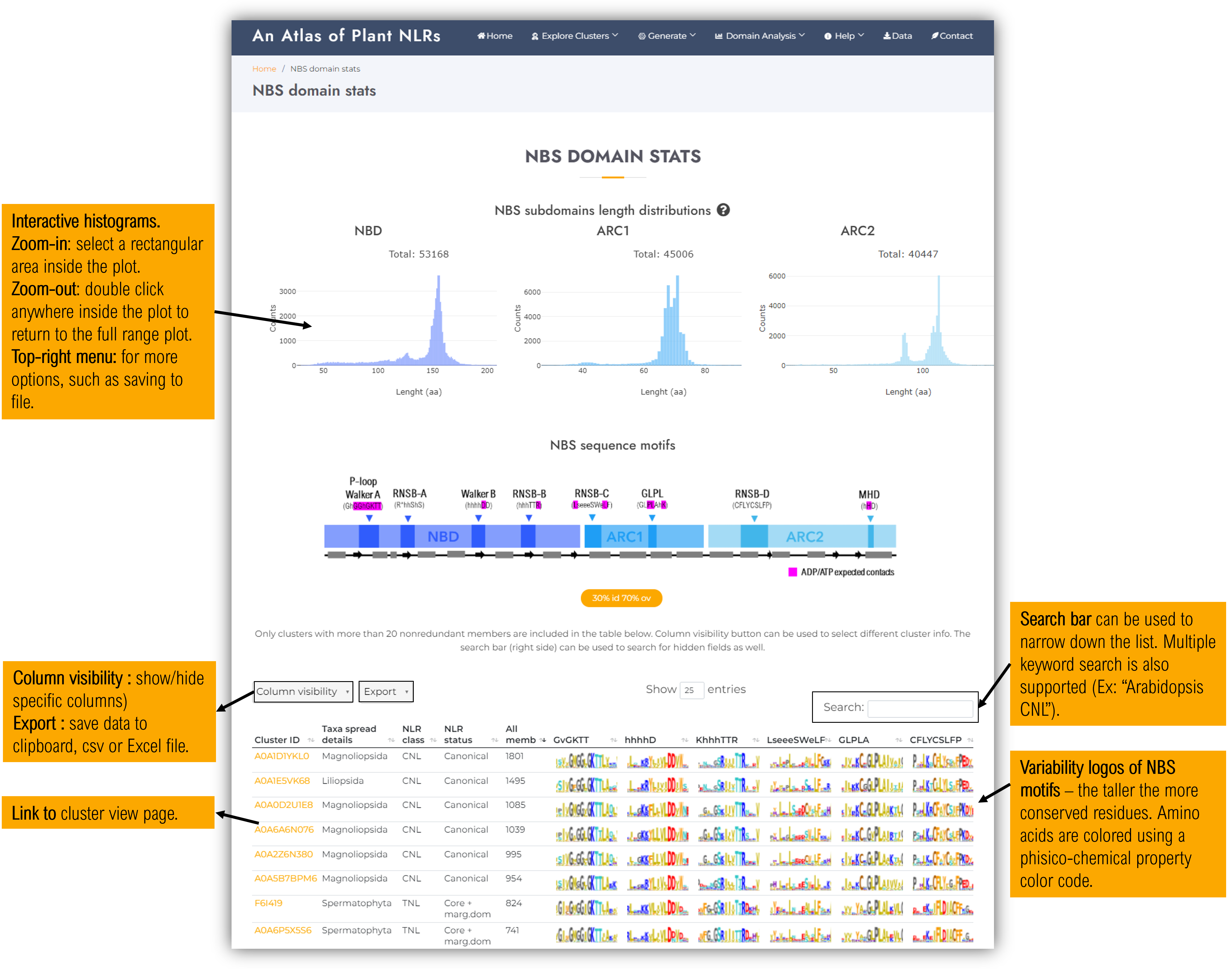
3. General domain statistics
3.1. NBS domain stats
Contains general statistics of the NBS domains present in the atlas:
- Interactive histograms of each subdomain length (aa).
- NBS motifs variability plots
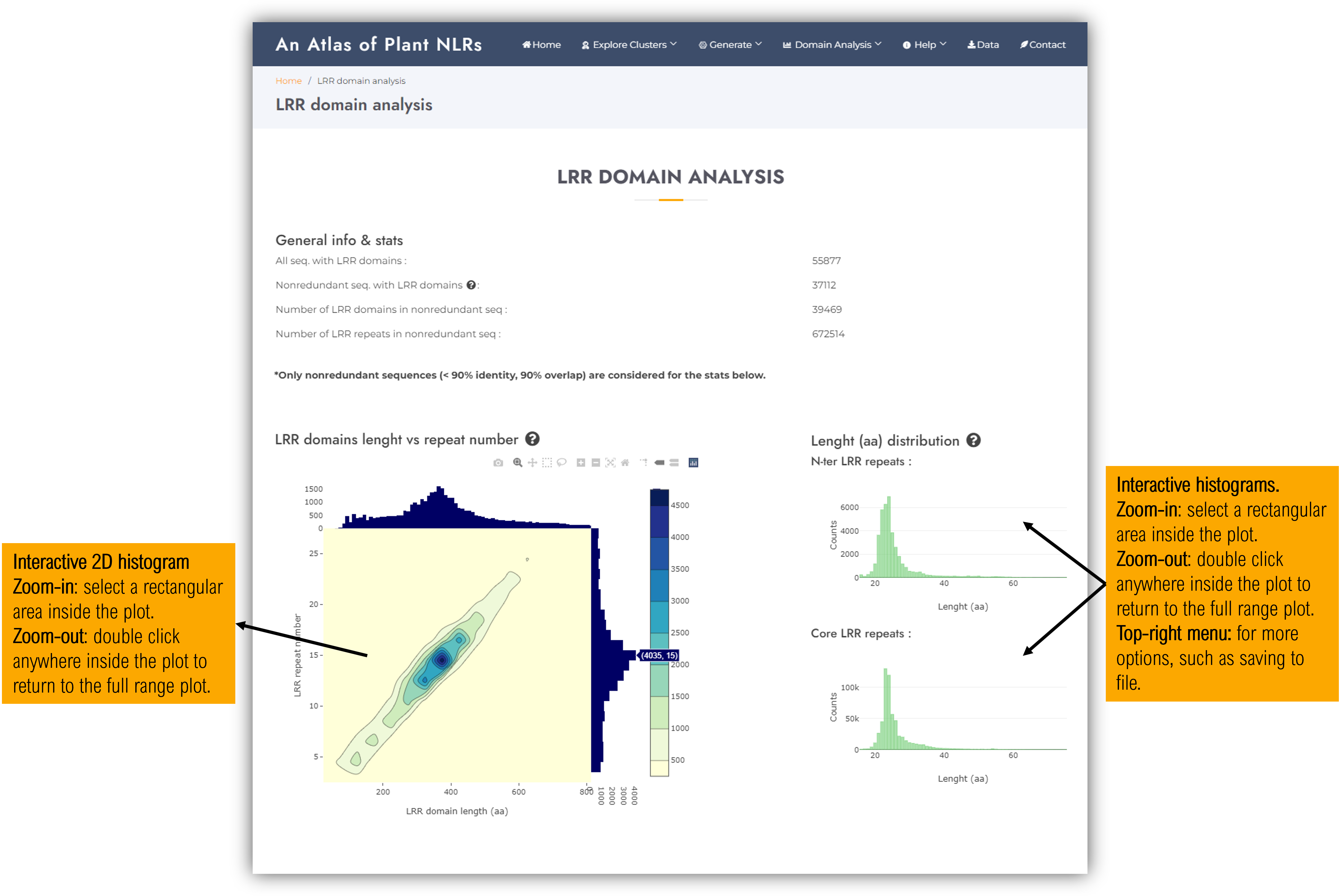
3.2. LRR domain stats
Contains general statistics of the LRR domains present in the atlas:
- Interactive 2D histograms of LRR domain length (aa) versus number of LRR repeats.
- LRR repeats length histograms of N-ter and core LRR repeats.
References
Potter, S. C., Luciani, A., Eddy, S. R., Park, Y., Lopez, R., & Finn, R. D. (2018). HMMER web server: 2018 update. Nucleic Acids Research, 46(W1), W200–W204.
https://doi.org/10.1093/nar/gky448
Mitchell, A. L., Attwood, T. K., Babbitt, P. C., Blum, M., Bork, P., Bridge, A., … Finn, R. D. (2019). InterPro in 2019: Improving coverage, classification and access to protein sequence annotations. Nucleic Acids Research, 47(D1), D351–D360.
https://doi.org/10.1093/nar/gky1100
Steinegger, M., & Söding, J. (2017). MMseqs2 enables sensitive protein sequence searching for the analysis of massive data sets. Nature Biotechnology 2017 35:11, 35(11), 1026–1028.
https://doi.org/10.1038/nbt.3988
Franz M, Lopes CT, Huck G, Dong Y, Sumer O, Bader GD. (2016). Cytoscape.js: a graph theory library for visualisation and analysis. Bioinformatics (2016) 32 (2): 309-311 first published online September 28, 2015
https://doi.org/10.1093/bioinformatics/btv557
Shannon P, Markiel A, Ozier O, et al. Cytoscape: a software environment for integrated models of biomolecular interaction networks. Genome Res. 2003;13(11):2498-2504.
https://doi.org/10.1101/gr.1239303
Yachdav, G., Wilzbach, S., Rauscher, B., Sheridan, R., Sillitoe, I., Procter, J., Lewis, S. E., Rost, B., & Goldberg, T. (2016). MSAViewer: interactive JavaScript visualization of multiple sequence alignments. Bioinformatics (Oxford, England), 32(22), 3501–3503.
https://doi.org/10.1093/bioinformatics/btw474
Wang, S., Peng, J., Ma, J., & Xu, J. (2016). Protein Secondary Structure Prediction Using Deep Convolutional Neural Fields. Scientific reports, 6, 18962.
https://doi.org/10.1038/srep18962
Wang, S., Li, W., Liu, S., & Xu, J. (2016). RaptorX-Property: a web server for protein structure property prediction. Nucleic acids research, 44(W1), W430–W435.
https://doi.org/10.1093/nar/gkw306
Martin, E. C., Sukarta, O., Spiridon, L., Grigore, L. G., Constantinescu, V., Tacutu, R., Goverse, A., & Petrescu, A. J. (2020). LRRpredictor-A New LRR Motif Detection Method for Irregular Motifs of Plant NLR Proteins Using an Ensemble of Classifiers. Genes, 11(3), 286.
https://doi.org/10.3390/genes11030286
Katoh, K., & Standley, D. M. (2013). MAFFT multiple sequence alignment software version 7: improvements in performance and usability. Molecular biology and evolution, 30(4), 772–780.
https://doi.org/10.1093/molbev/mst010
Tareen, A., & Kinney, J. B. (2020). Logomaker: beautiful sequence logos in Python. Bioinformatics (Oxford, England), 36(7), 2272–2274.
https://doi.org/10.1093/bioinformatics/btz921
Jumper, J., Evans, R., Pritzel, A. et al. Highly accurate protein structure prediction with AlphaFold. Nature 596, 583–589 (2021).
https://doi.org/10.1038/s41586-021-03819-2
Varadi M, Anyango S et al., AlphaFold Protein Structure Database: massively expanding the structural coverage of protein-sequence space with high-accuracy models, Nucleic Acids Research, Volume 50, Issue D1, 7, 2022, Pages D439–D444.
https://doi.org/10.1093/nar/gkab1061
Watkins X, Garcia LJ, Pundir S, Martin MJ; UniProt Consortium. ProtVista: visualization of protein sequence annotations. Bioinformatics. 2017 Jul 1;33(13):2040-2041.
https://doi.org/10.1093/bioinformatics/btx120.
Rego N, Koes D. 3Dmol.js: molecular visualization with WebGL. Bioinformatics. 2015 Apr 15;31(8):1322-4.
https://doi.org/10.1093/bioinformatics/btu829